Regression – Cost Function and Gradient Descent

Linear regression is an ML discipline, where one or more input features are mapped to a continuous output variable. A linear regression model is essentially a mathematical function that is learned from known data that maps input features to output labels, known as training data, which can then be used to predict output labels for new data. The learning algorithm looks at the training data set and learns the intercept and coefficients for the mathematical function.

An example for this is trying to predict house price based on information known about a house like the living area, the number of bedrooms, the number of floors, whether new or not etc. To be able to predict sale price, the ML algorithm looks at existing sales data, where both the attributes of the sold houses and the selling prices are known, to learn a model that maps the features to a price. This model can then be used to predict prices for houses newly coming on to the market.

Hypothesis Function

The machine learning model that is learned from the training data is called the hypothesis function. Let us say the problem we are trying to solve has n features, each feature indicated x1, x2, x3, …, xn, the hypothesis function is,

hϴ(x) = ϴ0 + ϴ1 * x1 + ϴ2 * x2 + ϴ3 * x3 + …. + ϴn * xn

Here ϴ0 is the intercept and ϴ1 through to ϴn are coefficients for each of the input features. If there are m samples in the training set, X is essentially a matrix of m x n + 1 dimension and ϴ is a column vector of size n + 1. So H(ϴ) is a matrix product of X and ϴ. So the objective of the learning algorithm is to learn the values of ϴ, based on the training data, that will fit well on the training data and generalize well for new data that is unknown.

Cost Function

Linear regression learns the coefficients is using something called a cost function. The cost function essentially operates on the deviation between the predicted values and actual values within the training set.

One of the popularly used cost function works on the residual mean square error, this is the mean of the square of the difference of predicted values and the actual value. If the actual value is indicated by the vector Y, the RMSE cost function is indicated as below,

J(ϴ) = 1 / 2m ∑ (hϴ(xi) – yi)² [i = 1 to m]

Leser the value of the cost function, better is the fit of the model to the training data. The objective of the learning exercise is to compute the values of ϴ that minimizes the value of J(ϴ).

Gradient Descent

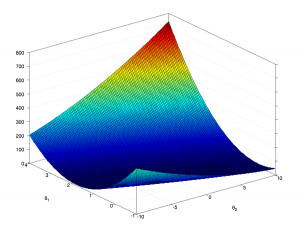
If we plot J(ϴ) against ϴ in a hyperplane, the resulting model will have a single global minimum value, that will correspond to the value of ϴ, where J(ϴ) is the minimum. Obviously, this is something difficult to visualize except using a contour plot. However, if we use a univariant model (a model with only one input feature), and plot J(ϴ) against ϴ in two dimensions, the resulting plot will be of the shape of a bowl, and the bottom most point of the plot representing the value of ϴ, where J(ϴ) is the minimum. The cost function for linear regression is a convex function, which essentially has one global minimum.

If we take the 3D plot above and create a contour plot, the optimal value of ϴ0 and ϴ1, to get the minimum value of the cost function will correspond to the middle of the innermost ellipses.

Gradient descent is an algorithm where we start with initial value(s) of ϴ, and go through a number of iterations, descending the gradient of the convex function, by adjusting the values of ϴ by a factor known as a learning rate, till the iterations converge, where the changes in J(ϴ) becomes less than an arbitrarily defined minimum value. Alternatively, you can keep adjusting the values of ϴ for a fixed set of iterations.

One way to do this is to take the gradient of the cost function curve at a given point and adjust the value of ϴ using the gradient multiplied by a learning factor. Higher up in the curve, the gradient will be higher and the algorithm will descend faster, once it starts reaching the optimal value the gradient will start decreasing with the gradient flattening out to zero at the minimal value of the cost function. The gradient of the cost function for a given ϴ (remember ϴ is not a scalar, but a vector with each element corresponding to the intercept and each input variable), is the partial derivative of the function with respect to a given ϴ.

The partial derivative of the cost function with regards to ϴ1, which is the coefficient of the input feature x1, will be.

1/m * ∑(hϴ(xi) – yi) * x1i [i = 1 to m]

So, the gradient descent algorithm will in each iteration update ϴ as follows

ϴ1 = ϴ1 – α/m * ∑(hϴ(xi) – yi) * x1i [i = 1 to m]

Gradient Descent Example

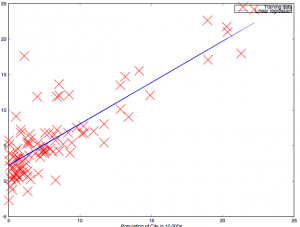
Now we will have a look at implementing gradient descent using simple Scala code. I have a dataset for a chain store that maps population in a given city to the profit that is made in that city, as a two-column CSV file. The snippet below reads the raw data from the file and maps each line to a three element tuple, the first element being a constant 1 corresponding to the intercept, the second being the input feature and the third being the output label.

val source = scala.io.Source.fromFile("price.txt")
val lines = source.getLines.map(_.split(",")).toList
val recs = lines.map(x => (1, x(0).toDouble, x(1).toDouble))

Now we define the function that implements the gradient descent logic.

def gradientDescent(t0: Double, t1: Double, it: Int, a: Double) : (Double, Double) = it match {
  case 0 => (t0, t1)
  case _ =>
    val x = t0 - recs.map(x => t0 + t1 * x._2 - x._3).reduce(_ + _) * a / recs.size
    val y = t1 - recs.map(x => (t0 + t1 * x._2 - x._3) * x._2).reduce(_ + _) * a / recs.size
    gradientDescent(x, y, it - 1, a)
}

Normal Equation

Rather than applying an iterative logic, we can use linear algebra to define a normal equation to solve the optimal values of ϴ, as we know at the point of the minimal value of the cost function, the gradient with respect to each ϴ, and consequentially the partial derivative is zero. We will look into this in detail in the next post.