
ML Linear Regression – Primer
Linear regression is one of the most basic tools used for predictive analysis. In this post we will look at some of the key concepts behind linear regression and look at performing linear regression to perform predictive analysis using Apache Spark Machine Learning library.
Linear regression is a supervised technique, where known relationship between a sample space of two continuous variables are used to derive intelligence to predict the value of one of the variables based on the value of the other. The variable that is predicted is called by a number of different terms including response, dependent variable, observation, outcome etc. The variable whose value is used to predict the response is called the independent, explanatory or predictor variable.
Simplistic Approach
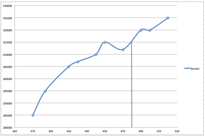
Let us take an example of predicting house prices. As a starting point, we take historic house sales data, and we try to base our prediction on the relationship between the square footage of each sold house against the sales price. A statistical starting point would be to plot the house prices against the square footage and find an observation that matches the square footage of the house, whose value we are trying to predict.
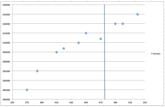
If we try to find an observed point on the above plot, for a square footage for which we want to predict the price, it may be likely we won’t find an exact match. The next step would be to find a range for the square footage and try to find sold prices within that range. Though, with that approach we are missing out on majority of the recorded observations to draw intelligence to form the prediction.
Building a Model
The obvious next step is to model an equation comprising the recorded observations and try to predict the price based on that model, as shown below.
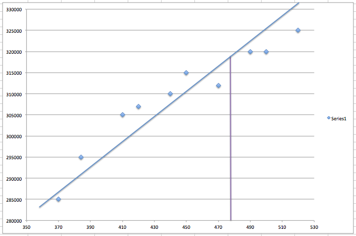
That looks like a sensible approach. The straight-line graph above is represented by an intercept on the Y axis and a slope, which is often expressed a f(x) = w0 + w1*x. Here the constants w0 and w1 are called regression parameters.
Evaluating Regression Error
However, how do we know whether the chosen values for w0 and w1 are the most optimal values for our model? One way of quantifying this is Residual Sum of Squares (RSS). Here we take the difference in the predicted value for each observation and the actual value, square the difference and sum them up for all the observations.
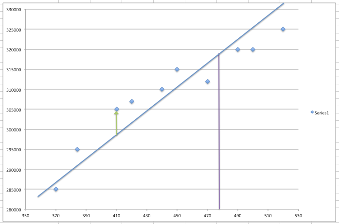
The fitness of the model is indicated by the least value of the RSS. Another matrix that is often used is the Root Mean Squared Error (RMSE), which is the square root of the mean of RSS.
Best fit Vs Over fit
However, the most optimal model may not be a linear relationship. It could be a quadratic fit for example, where f(x) = w0 + w1*x + w2*x*x.
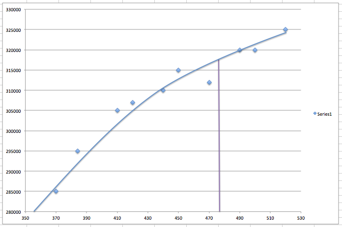
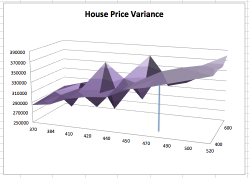
The best way to reduce the RMSE to zero, is to created an nth order polynomial model, where every single observation fits into the model, as shown below.
The above model will bring RMSE to zero. However, is definitely not going to be the most optimal model for predictions. In our example, the slight outlay in the observation on the left (corresponding to the square footage of 470), would skew the curve against us. This phenomenon is called over-fit of the model, where it doesn’t reflect the reality in terms of predicting the unknown.
Multiple Predictors
In our example, we have only looked at the square footage as the predictor. However, there could be more than one independent variable, like the land area, number of bedrooms, general condition of the property etc. These variables may either be continuous or discrete. In this instance, the model becomes a multi-dimensional plane, instead of a line as shown below including the lot area as a second independent variable, and could be represented as, for example, f(x, y) = w0 + w1*x + w2*y.
Model Evaluation
One way of evaluating the accuracy of the model is to split the data into training and test samples. The regression algorithm will be trained with the training dataset to generate an optimal model with an optimal RMSE, and the model can then be evaluated against the test dataset.
Applying the Theory
Now we will use Apache Spark to apply the theory we have covered so far in this post. The data file used for this example can be downloaded here. We use Spark SQL to first load the comma-separated data as below into a data frame as below, and print the schema.
scala> val df = spark.read.
     | option("header", "true").
     | option("inferSchema", "true").
     | csv("home_data.csv")

scala> df.printSchema
root
 |-- id: long (nullable = true)
 |-- date: string (nullable = true)
 |-- price: integer (nullable = true)
 |-- bedrooms: integer (nullable = true)
 |-- bathrooms: double (nullable = true)
 |-- sqft_living: integer (nullable = true)
 |-- sqft_lot: integer (nullable = true)
 |-- floors: double (nullable = true)
 |-- waterfront: integer (nullable = true)
 |-- view: integer (nullable = true)
 |-- condition: integer (nullable = true)
 |-- grade: integer (nullable = true)
 |-- sqft_above: integer (nullable = true)
 |-- sqft_basement: integer (nullable = true)
 |-- yr_built: integer (nullable = true)
 |-- yr_renovated: integer (nullable = true)
 |-- zipcode: integer (nullable = true)
 |-- lat: double (nullable = true)
 |-- long: double (nullable = true)
 |-- sqft_living15: integer (nullable = true)
 |-- sqft_lot15: integer (nullable = true)
Spark ML library works with notion of labeled points, which is essentially a map of one or more features expressed as a vector against the recorded observation. We start with a simple model that maps the data frame to a list of labeled points and split the data into 80% training and 20% test.
scala> import org.apache.spark.ml.feature.LabeledPoint
import org.apache.spark.ml.feature.LabeledPoint

scala> import org.apache.spark.ml.linalg.Vectors
import org.apache.spark.ml.linalg.Vectors

scala> import org.apache.spark.ml.regression.LinearRegression
import org.apache.spark.ml.regression.LinearRegression

scala> val Array(training, test) = df.map {r =>
     | new LabeledPoint(r.getInt(2), Vectors.dense(r.getInt(5)))
     | }.randomSplit(Array(0.8, 0.2), 1)
Then we create a regression model using the training data, and use the resultant model to predict the test data and print the actual and predicted values for comparison. We also print the RSS and RMSE when the model is applied on the test data set.
scala> val lr = new LinearRegression()
lr: org.apache.spark.ml.regression.LinearRegression = linReg_83b7a5c545b7

scala>   val model = lr.fit(training)

scala>   model.transform(training).show(10)
+-------+--------+------------------+
|  label|features|        prediction|
+-------+--------+------------------+
|75000.0| [670.0]| 152002.7922210247|
|78000.0| [780.0]|182264.89866576367|
|80000.0| [430.0]| 85976.37815977602|
|81000.0| [730.0]|168509.39573633685|
|82500.0| [520.0]|110736.28343274427|
|83000.0| [900.0]|  215278.105696388|
|84000.0| [700.0]|160256.09397868076|
|85000.0| [830.0]|196020.40159519046|
|85000.0| [910.0]|218029.20628227334|
|89000.0| [900.0]|  215278.105696388|
+-------+--------+------------------+
only showing top 10 rows

scala> val rmse = model.evaluate(test).
     | rootMeanSquaredError
rmse: Double = 277584.74524589145
If you want to build a more complex model, that takes additional features, you can do as well. As will see, more features don’t essentially mean better predictions. However, if you have outliers which shift the value because of some peculiar feature, like renovations or house being on the waterfront, it is likely to get a better prediction by adding more features.

That insight solves the prboelm. Thanks!